Multiple Solutions System of Equations Matlab
In this tutorial, a block diagram is designed which will help us to solve a system of linear equations using MATLABs' Simulink. At the start a brief introduction to a linear equations and system of linear equations are provided. After that a simple example is performed on MATLAB simulink in which a sample system of linear equations is taken and I solved for the variables involved with the help of simulink. The example taken here is to solve two linear equations for two unknowns we can however extend it for solving larger number of equations simultaneously. At the end a simple exercise is provided regarding the concepts and blocks used in this tutorial.
Introduction to linear equation and system of linear equations
A linear equation is a mathematical term which is in the form of unknown variables whose power is one and which can be written in the form of point slope equation as given below,
y=mx+c
Where m is the slope of the line and c is the y-intercept. The graph of a linear equation is a straight line. A system of linear equations is, however, a set of linear equations which contains same variable. The number of equations is equal to the number of unknowns present in the equation. For instance, if the system contains 5 linear equations then the number of unknown or variables in all these equations collectively is also 5 with each equation satisfying the definition of linear equations (having the power of each variable equal to 1). In this tutorial we are going to solve a system of linear equations with two equations and two unknowns and the equations are given below,
2x+3y = -4
4x+5y = -5
Lets' suppose the general system was
a1*x + b1 * y = -k1
a2*x + b2 * y = -k2
This implies that a1 = 2, b1 = 3, k1 = 4, a2 = 4, b2 = 5, k2 = 5
These values will be used in the tutorial later.
How to solve linear equations with Simulink
Lets' now move towards a simple example for solving the system of linear equations using Simulink. In Simulink a block named as Algebraic Constraint will help us do the job for us. However, it is not that simple we also have to apply some logic in order to solve the system of linear equations. Lets' now begin with the programming part. Open MATLAB and then Simulink as we have done in previous tutorials. After that open the library browser and from the library browser select the commonly used blocks as we have been doing in previous tutorials. From that section select the gain block and drag and drop that gain block on the simulink block diagram section. Place two such gain blocks as the example we have taken here is for two unknown variables, as shown in the figure below,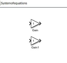
Figure 1: Gain blocks
- These gain blocks are used to enter the value of the co-efficient of each of the variables, hence the number of gain blocks is equal to the number of unknowns in the equation. As we are using a system of equations with two unknowns hence the number of gain blocks is two.
- Next comes the constant part. The constant at the right hand side of the equation can be placed in the block diagram in the form of a constant block. From the commonly used blocks section in the library browser of simulink, select the block of a constant and place it with the two already placed gain blocks as shown in the figure below,
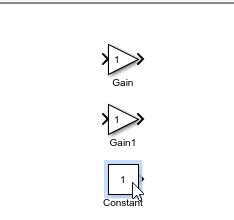
Figure 2: Constant block
- Now what we need to do is to add all these three blocks. To do so we can also use the sum block but as we are interested in exploring more blocks in simulink we will use another block provided by simulink to add up things together. From the library browser click on the Math operations section as shown in the figure below,

Figure 3: Math operations
- From this section select the add block as shown in the figure below,
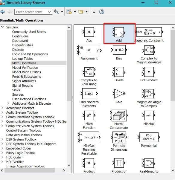
Figure 4: Add block
- This add block will do the same job as the sum block we have used in previous tutorials. As you can see the number of inputs provided by this add block is two, however, we want to add up three things together (two gain blocks and one constant) we thus now need to update the parameters of add block. Double click on the add block, and in the list of signs add a + sign to increase the number of inputs as shown in the figure below,
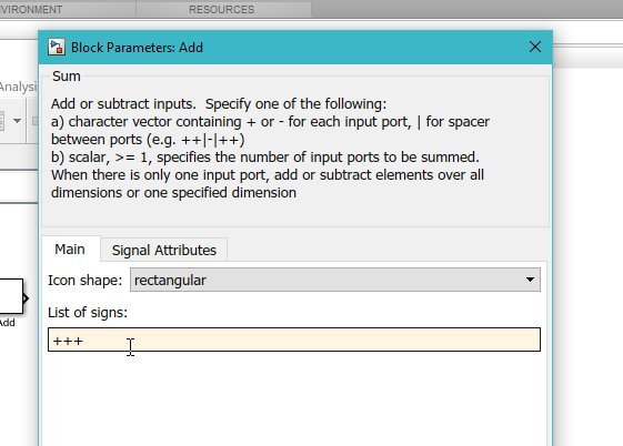
Figure 5: List of signs
- At the input of the add block connect all the already placed blocks i.e. two gain blocks and a constant with the help of a wire as shown in the figure below,
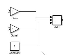
Figure 6: Adding
- This is the adder of equation 1 so we will name the gain and constant as a1, b1 and k1. The next step here is to place an Algebraic constraint block. This constraint block inputs a function whose input should be equal to zero and estimates the output of the functions value. The output of the block must be provided to the input co-efficient through a feedback loop and with each iteration the output value will be updated until we receive a correct value for that unknown. The initial value provided to the constraint block is zero here. From the math operations section select the Algebraic constraints block as shown in the figure below,
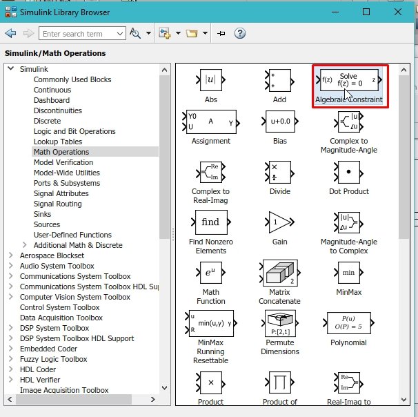
Figure 7: Algebraic constraints
- At the input of that block connect the output of the adder. Now select the sinks section from the library browser of simulink as shown in the figure below,
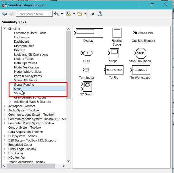
Figure 8: Sinks
- From this section select the display block as shown in the figure below,
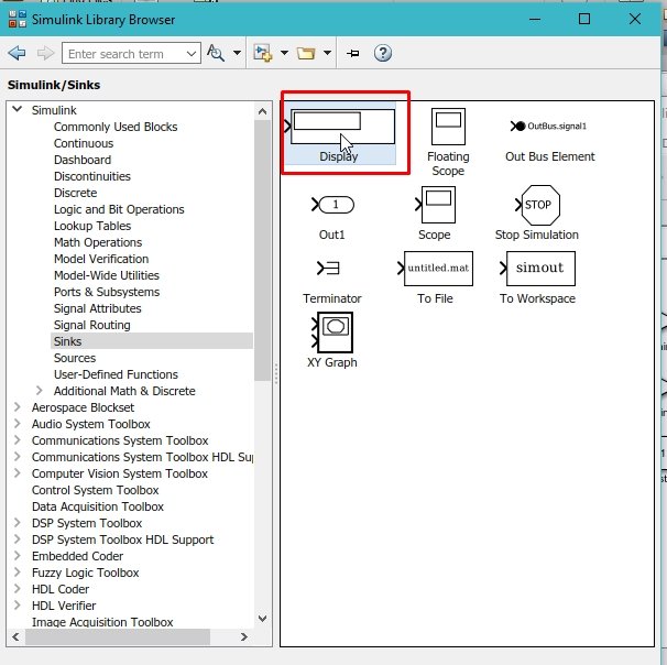
Figure 9: Display
- Place this block at the output of the constraint block. This block is used to display the output of the program. We have now designed a complete block diagram of one of the equation as shown in the figure below,

Figure 10: Block diagram of one equation
- Simply copy and paste this complete block diagram to get the block diagram of second equation as shown in the figure below,
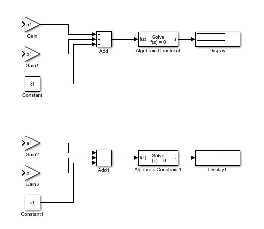
Figure 11: Block diagrams for both equations
- Update the variable names of the second block as a2, b2 and k2. Now comes the part of connecting the feedback to the constraint block. Connect the feedback wire from the output of the 1st constraint block to the input of block a1 and a2 as these are the co-efficient of x (which will be displayed in 1st constraint block, as shown in the figure below,
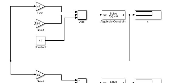
Figure 12: X value
- Do the same with 2nd constraint block and b1, b2 as shown in the figure below,
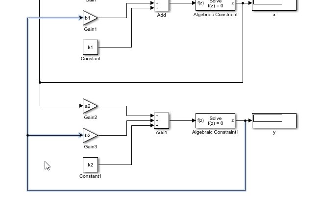
Figure 13: Y value
- The highlighted wires show the feedback path for y value. Now go back to the MATLAB command window where we will define the values of the variables as shown in the figure below,
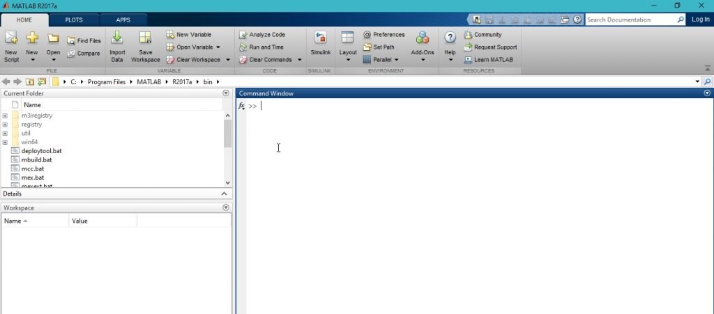
Figure 14: Command window
- Define all the values of the variables in the command window as we have given in the introduction portion as shown in the figure below,
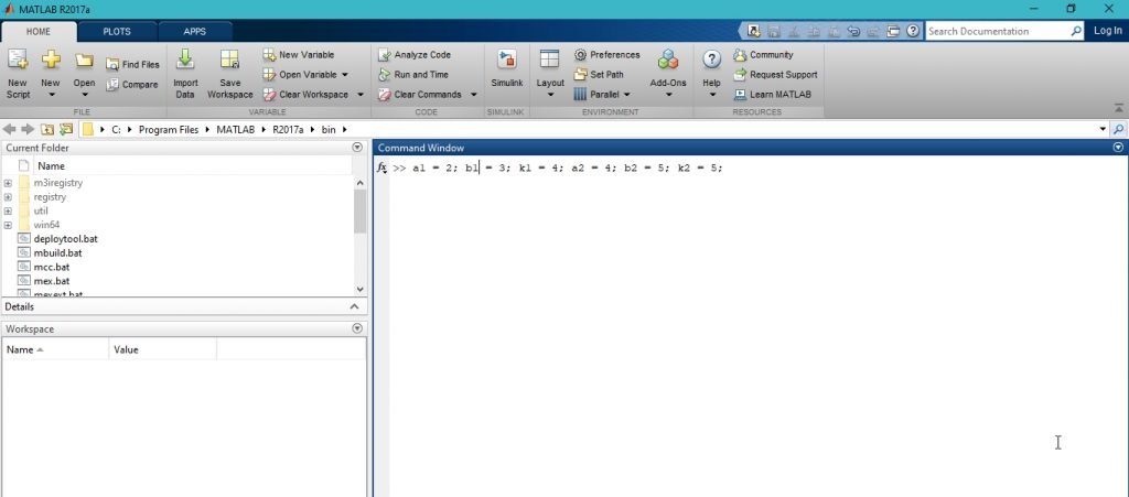
Figure 15: Variable value assignment
- After you run the command, these variables will appear in the workspace of MATLAB which can be accessed in Simulink also as shown in the figure below
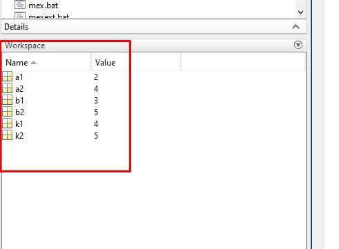
Figure 16: Workspace
- Run the simulink block diagram now from the run icon on the screen and the output of the solution of system of linear equations will be displayed in the display box as shown in the figure given below,

Figure 17: Output
Exercise:
- Design a block diagram that will be able to solve three linear equations with three unknowns as provided in the equations given below,
3x+4y-2z=9 ; 5x+2y+z=0 ; x-y+5z=11
Multiple Solutions System of Equations Matlab
Source: https://microcontrollerslab.com/solving-linear-equations-simulink/